Research
Selected publications
Londschien M., Burger M., G. Rätsch, and Bühlmann P. (2026) Domain generalization and adaptation in intensive care with anchor regression, RSS Data Science and Artificial Intelligence
Londschien M. and Bühlmann P. (2026) Weak-instrument-robust subvector inference in instrumental variables regression: A subvector Lagrange multiplier test and properties of subvector Anderson-Rubin confidence sets, Journal of Econometrics
Londschien M. (2025) A statistician’s guide to weak-instrument-robust inference in instrumental variables regression with illustrations in Python, arXiv
Burger M., Chopard D.*, Lichtner G.*, Londschien M.*, Sergeev F.*, Fuchs M., Yèche H., Kuznetsova R., Faltys M., Gerdes E., Leshetkina P., Christ M., Schanz M., Göbel N., Bühlmann P., Grünewald E., Balzer F., and Rätsch G. (2025) A foundation model for intensive care: Unlocking generalization across tasks and domains at scale, medRxiv
Londschien M., Bühlmann P. and Kovács S. (2023) Random Forests for Change Point Detection, Journal of Machine Learning Research
Domain generalization and adaptation in intensive care with anchor regression
Londschien M., Burger M., Rätsch G. and Bühlmann P. (2026), RSS: Data Science and Artificial Intelligence
Predictive models in clinical settings often suffer significant performance drops when deployed in new hospitals due to distribution shifts. Distributional robustness methods developed to address this largely succeed only on synthetic or highly curated datasets, often failing to outperform simple baselines in large-scale empirical studies.
We leverage causal models to exploit existing data heterogeneity. The core intuition is that true causal relationships (e.g., administering a vasopressor raises blood pressure) remain stable across different domains, whereas relationships driven by hidden confounding (e.g., vasopressor use correlating with increased mortality because clinicians only prescribe it to the sickest patients) shift when treatment policies change. We use anchor regression, which promotes stability by penalizing dependencies that vary with a designated “anchor” variable $A$.
As linear models are unable to capture the feature interactions inherent in clinical data, we developed anchor boosting, a novel tree-based nonlinear extension of anchor regression optimized using second-order updates. Let $A$ be the anchor variable encoding data heterogeneity and $P_A := A (A^T A)^{-1} A^T$ be the linear projection onto the column span of $A$. The anchor loss is \(\ell(f, y) = 0.5 \| y - f \|^2 + 0.5 (\gamma - 1) \| P_A (y - f) \|^2,\) where $\gamma$ controls the amount of causal regularization. This has gradient $g(f,y) = - (y - f) - (\gamma - 1) P_A (y - f)$ and Hessian $H(f, y) = \mathrm{Id} + (\gamma - 1) P_A$ with respect to $f$. Let $\hat f^j$ be the learner after $j$ steps of boosting. We then fit the loss’ negative gradient against the features $X$ using a decision tree $\hat t^{j+1} := - g(f, y) \sim X$. Let $M \in \mathbb{R}^{n \times \mathrm{num. leaves}}$ be the one-hot encoding of $\hat t^{j+1}$’s leaf node indices. Then, $M^T g(\hat f^j(X), y)$ and $M^T H(\hat f^j(X), y) M$ are the gradient and Hessian of the loss $\ell(\hat f^j(X) + \hat t^{j+1}(X), y) = \ell(\hat f^j(X) + M \hat \beta^{j+1}, y)$ with respect to $\hat t^{j+1}$’s leaf node values $\hat \beta^{j+1} \in \mathbb{R}^{n \times \mathrm{num. leaves}}$. We set them using a second order optimization step
\[\hat \beta^{j+1} = - (M^T H(\hat f^j(X), y) M)^{-1} M^T g(\hat f^j(X), y)\]For classification, we replace the MSE with the probit loss and use score residuals, equal to the loss’ gradient with respect to $f$. In our experiments we found that three factors are essential for anchorboosting’s ability to improve out-of-distribution performance: (i) second-order optimization of tree leaf values, (ii) using the probit loss instead of the logistic loss for classification, and (iii) sufficiently regularizing tree fitting by limiting the maximum depth or number of leaves.
We applied linear anchor regression and our anchor boosting to predict adverse events using a massive dataset of 10 million observations from 400,000 patients aggregated across nine distinct intensive care unit (ICU) databases. This is the largest application of a causality-inspired method to a medical prediction problem. We empirically establish the following: (i) Anchor regularization improves predictive performance when applied to data from ICUs not seen during training. This is a significant success given the overwhelmingly negative results of prior domain generalization methods on ICU data. (ii) The performance gains are largest for the most dissimilar, truly out-of-distribution target domains. (iii) Selecting the causal regularization parameter $\gamma$ remains difficult. (iv) Conventional hyperparameter selection is critical. Even for simpler linear anchor regression, adding an elastic-net regularization term was essential to improve OOD performance. We observe a strong interaction between the optimal amounts of causal and conventional regularization. (v) Both anchor methods appear to be robust to some violations of the anchor exogeneity assumption, an important consideration for practitioners without access to purely exogenous variables.
Finally, we propose a practical conceptual framework to quantify the utility of large external datasets when target-domain data is limited. When few samples from the target domain are available, we refit the linear and tree-based models in an empirical Bayes fashion. By evaluating model performance as a function of the available target sample size, we identify three distinct operational regimes:
- Domain generalization regime: Target data is heavily restricted. Only the external model should be used.
- Domain adaptation regime: Moderate target data is available. Refitting the external model yields the best results.
- Data-rich regime: Target data is abundant. Training strictly on target data is optimal, and external data provides no additional value.
Weak-instrument-robust subvector inference in instrumental variables regression: A subvector Lagrange multiplier test and properties of subvector Anderson-Rubin confidence sets
Londschien M. and Bühlmann P. (2026), Journal of Econometrics.
Instrumental variables regression (IV) is a method for causal effect estimation when controlled experiments are infeasible. If the explanatory variable of interest is correlated with the error term (endogenous), standard regression techniques such as ordinary least squares (OLS) yield biased estimates for the causal effect. IV uses instruments, variables that are correlated with the explanatory variable but not with the error, to isolate variation in the explanatory variable of interest that is uncorrelated with the error term, to yield an unbiased estimate of the causal effect.
To influence policy, uncertainty quantification is essential. Typically, Wald tests based on the estimator’s asymptotic normality are used to construct confidence sets and p-values. In many applications of IV, the signal-to-noise ratio in the first stage, from the instruments to the explanatory (endogenous) variable of interest, is low, leading Wald-based confidence sets to undercover.
An alternative are tests that are robust to such weak instruments.
The Anderson-Rubin test is one option. It has the correct size independently of instrument strength and confidence sets obtained by test inversion have a closed-form solution. However, the degrees of freedom of the limiting chi-squared distribution are equal to the number of instruments, not the number of tested parameters. Consequently, adding instruments might lead to larger confidence sets.
Another weak-instrument-robust test is Kleibergen’s (2002) Lagrange multiplier test. The degrees of freedom of its limiting chi-squared distribution equal the number of parameters under test. Consequently, adding instruments should only improve identification and result in smaller confidence sets.
If there are multiple endogenous variables, confidence sets for the entire parameter vector are difficult to interpret. Subvector confidence sets for individual coefficients of the causal parameter are more useful. Guggenberger et al. (2012) propose a subvector variant of the Anderson-Rubin test by plugging in the LIML (the MLE assuming Gaussian noise) for the nuisance parameter. In the same paper they also show that the similarly obtained subvector variant of the Lagrange multiplier test has incorrect size.
In our work, we
- propose a subvector variant of the Lagrange multiplier test by minimizing over the nuisance parameter. We show that this has the correct size under a technical condition. This is the first weak-instrument-robust subvector test in instrumental variables regression to recover the degrees of freedom of the (not weak-instrument-robust) Wald test.
- We compute the closed-form solution for the confidence sets obtained by inverting the (subvector) Anderson-Rubin test. We show that the $1 - \alpha$ subvector confidence sets for an individual parameter are jointly bounded if and only if Anderson’s (1951) likelihood ratio test that the first-stage parameter is of reduced rank rejects at level $\alpha$. The confidence sets are centered around a k-class estimator and, if bounded and non-empty, equal a Wald-based confidence set around that estimator.
Our test fills a gap in the weak-instrument-robust testing literature for instrumental variables regression:
| Anderson-Rubin | Lagrange multiplier | conditional likelihood-ratio | |
|---|---|---|---|
| complete | Anderson and Rubin (1949) | Kleibergen (2002) | Moreira (2003) |
| subvector | Guggenberger et al. (2012) | us | Kleibergen (2021) |
Let $k = \mathrm{dim}(Z)$ be the number of instruments and $m \leq k$ be the number of endogenous variables. Subvector tests are for a single parameter.
| degrees of freedom | subvector DOF | weak-instrument-robust? | closed-form confidence set? | possibly unbounded? | |
|---|---|---|---|---|---|
| Wald | $m$ | $1$ | no | yes | no |
| likelihood-ratio | $m$ | $1$ | no | yes | yes |
| Anderson-Rubin | $k$ | $k - m + 1$ | yes | yes | yes |
| conditional likelihood-ratio | in-between | in-between | yes | no | yes |
| Lagrange multiplier | $m$ | $1$ | yes | no | yes |
I implemented all the (subvector) tests mentioned above and the (subvector) confidence sets obtained by test inversion in the open-source Python software package ivmodels. See also the docs. This also implements k-class estimators, such as the two-stage least-squares (TSLS), limited information maximum likelihood (LIML), and Fuller estimators, and auxiliary tests such as the J-statistic of overidentification and Anderson’s (1951) likelihood-ratio test of reduced rank. A summary containing estimates, test statistics, p-values, and confidence sets can be generated with the k-class estimator’s summary method. ivmodels is available on conda-forge and pypi.
See also the examples in the docs:
- Card (1995): Using Geographic Variation in College Proximity to Estimate the Return to Schooling
- Tanaka, Camerer, and Nguyen (2010): Risk and Time Preferences: Linking Experimental and Household Survey Data from Vietnam
- Angrist and Krueger (1993): Does Compulsory School Attendance Affect Schooling and Earnings?
- Acemoglu, Johnson, Robinson (2001): The Colonial Origins of Comparative Development: An Empirical Investigation
A statistician’s guide to weak-instrument-robust inference in instrumental variables regression with illustrations in Python
Londschien M. (2025), arXiv
Instrumental variables regression (IV) is a method for causal effect estimation when controlled experiments are infeasible. If the explanatory variable of interest is correlated with the error term (endogenous), standard regression techniques such as ordinary least squares (OLS) yield biased estimates for the causal effect. IV uses instruments, variables that are correlated with the explanatory variable but not with the error, to isolate variation in the explanatory variable of interest that is uncorrelated with the error term, to yield an unbiased estimate of the causal effect.
The economics community has developed an extensive literature on estimation and uncertainty quantification in IV regression. These results are often missing from standard statistics curricula. Despite a recent surge of interest in causal inference and IV among statisticians, many such results and their proofs (e.g., the limited information maximum likelihood, LIML, estimator minimizes the Anderson-Rubin test statistic) are absent from statistical textbooks and overview papers.
This manuscript translates standard econometric results into a unified language accessible for mathematicians and statisticians.
Specifically, this guide covers:
- k-class estimators: Including OLS, two-stage least-squares (TSLS), and the LIML.
- Weak-instrument-robust inference: Including the Anderson-Rubin, conditional likelihood-ratio, and Lagrange multiplier tests, along with their partial (subvector) variants.
- Auxiliary tests: Such as the J-statistic for overidentification, the Cragg-Donald test for reduced rank, and residual prediction tests for misspecification.
Crucially, all estimators and tests introduced in the manuscript are implemented in the open-source Python package ivmodels. The paper walks through these methods step-by-step, illustrating the results using Card’s (1995) classic dataset estimating the causal effect of education on wages.
Summary
Model: Let $y_i = X_i \beta + \varepsilon_i$ and $X_i = Z_i^T \Pi + V_{X, i}$ for random $Z_i$, $V_{X,i}$ and $\varepsilon_i$ for $i=1, \ldots n$ and let $y \in \mathbb{R}^n, X \in \mathbb{R}^{n \times m_x}$, and $Z \in \mathbb{R}^{n \times k}$ be the stacked outcomes, endogenous covariates, and instruments (Model 1). Write $P_Z = Z (Z^T Z)^{-1} Z^T$ and $M_Z = \mathrm{Id} - P_Z$ be the orthogonal projection onto the column space of $Z$ and its orthogonal complement. In strong instrument asymptotics, $\Pi$ is constant and of full rank. In weak instrument asymptotics, $\Pi = \Pi_n = 1/\sqrt{n} C$ for some $C$ of full rank. Both imply $m_X \geq k$. We assume $Z^T (\varepsilon \ V_X)$ satisfies some central-limit theorem condition (Assumption 1), satisfied if the $Z_i, V_{X, i}, \varepsilon_i$ are i.i.d. with reasonable second moments (Lemma 1).
Estimators: The limited information maximum likelihood (LIML) estimator is the maximum likelihood estimator for the causal parameter assuming Gaussian error terms (Def. 6). Let \(\mathrm{AR}(\beta) = \frac{n-k}{k} \frac{\|P_Z (y - X \beta)\|^2}{\| M_Z (y - X \beta) \|^2}\) be the Anderson-Rubin (AR) test statistic (Def. 8). After marginalization of the nuisance parameters, the Gaussian IV likelihood equals $\mathrm{const} - \frac{n}{2} \log\Big(1 + \frac{k}{n-k} \mathrm{AR}(\beta) \Big)$ (Lem. 7). The LIML thus minimizes the AR test statistic (Cor. 9). K-class estimators $\hat\beta_\mathrm{k}(\kappa)$ (Def. 2) are minimizers of \(\beta \mapsto \kappa \| P_Z(y - X \beta) \|^2 + (1 - \kappa) \| y - X \beta \|^2\) for $\kappa \geq 0$ (Prop 3). Thus $\hat\beta_\mathrm{k}(0)$ is the ordinary least-squares (OLS), $\hat\beta_\mathrm{k}(1)$ is the two-stage least-squares (TSLS) estimator (Def. 4), and anchor regression estimators $\hat\beta_\mathrm{anchor}(\gamma) = \hat\beta_\mathrm{k}(\frac{\gamma - 1}{\gamma})$ for $\gamma \geq 1$. Under strong instrument asymptotics, a series of k-class estimators $\beta_\mathrm{k}(\kappa_n)$ are consistent if $\kappa \to_P 1$ and asymptotically normal if $\sqrt{n} (\kappa - 1) \to_P 0$ (Prop. 5). The LIML is a k-class estimator with data-dependent \(\kappa = \hat\kappa_\mathrm{LIML} = \lambda_\mathrm{min} \Big( \big[ (y \ X) M_Z (y \ X) \big]^{-1} \big[ (y \ X) P_Z (y \ X ) \big] \Big) + 1 \geq 1\) and $\hat\kappa_\mathrm{LIML} = \frac{k}{n-k} \mathrm{AR}(\hat\beta_\mathrm{LIML}) = \frac{k}{n-k} \min_\beta \mathrm{AR}(\beta)$ (Prop 10). If $k = m_x$, that is, there are as many instruments as endogenous covariates and the causal parameter is just-identified, then $\hat\kappa_\mathrm{LIML} = 1$ and $\hat\beta_\mathrm{LIML} = \hat\beta_\mathrm{TSLS}$ (Cor. 11). The LIML can also be interpreted as the TSLS estimator using “decorrelated” covariates $\tilde X(\hat\beta_\mathrm{LIML})$ for $\tilde X(\beta) := X - (y - X \beta) \frac{ (y - X \beta)^T M_Z X }{(y - X \beta)^T M_Z (y - X \beta)}$ (Prop. 12). The Fuller estimators are $\beta_\mathrm{Fuller}(\alpha) = \beta_\mathrm{k}(\hat\kappa_\mathrm{LIML} - \alpha / n)$.
Tests: Various tests exist for the causal parameter of interest. If there are multiple endogenous regressors ($m_X > 1$), practitioners are typically not only interested in tests for the entire causal parameter $\beta_0$, but rather in partial or subvector tests for individual components. To model this, we split $X$ into $X \in \mathbb{R}^{n \times m_X}, W \in \mathbb{R}^{n \times m_W}$ and $\beta_0$ into $(\beta_0, \gamma_0)$, where $X$ includes the endogenous regressors whose causal effect $\beta_0$ we wish to make inference for.
Under strong instruments asymptotics, we can use the Wald test applied to k-class estimators satisfying $\sqrt{n} (\kappa_n - 1) \to_P 0$ to make inference on $\beta_0$ (Def. 13, Prop. 14, Cor. 15). This covers the TSLS and, as we will see next, the LIML.
The subvector (partial) Anderson-Rubin test is obtained by splitting $\beta = (\beta, \gamma)$ and then minimizing over the nuisance parameter $\gamma$: $\mathrm{AR}(\beta) = \min_\gamma \mathrm{AR}(\beta, \gamma) = \mathrm{AR}(\beta, \hat\gamma_\mathrm{LIML})$, where $\hat\gamma_\mathrm{LIML}$ is the LIML using covariates W and outcomes $y - X \beta$ (Def. 17). Under both strong and weak instrument asymptotics, the subvector AR is bounded from above by a $\chi^2(k - m_W) / (k - m_W)$ distributed random variable (Prop. 18). Thus, it can be used to make weak-instrument robust inference on $\beta_0$ (Cor. 20). This also implies that $(n-k) (\hat\kappa_\mathrm{LIML} - 1) \leq \chi^2(k - m_X - m_W)$ (Cor. 19) and thus that, under strong instrument asymptotics, the LIML is asymptotically Gaussian.
The subvector AR has one drawback: It has $k - m_W - m_X$ “excess” degrees of freedom that do not test the “goodness of fit” of $\beta$ but rather so-called overidentifying restrictions, that is, whether overall model assumptions are met. Essentially, $\mathrm{AR}(\beta) = (\mathrm{AR}(\beta) - \min_b \mathrm{AR}(b)) + \min_b \mathrm{AR}(b) = (k - m_W) \mathrm{LR}(\beta) + (k - m_W) J_\mathrm{LIML},$ where $\mathrm{LR}$ is the likelihood-ratio test statistic for $\beta$ and the LIML variant of the J or Sargan-Hansen test statistic $J_\mathrm{LIML}$ tests misspecification. Consequently, a little bit of misspecification improves the power of the AR test and results in smaller confidence sets by increasing $J_\mathrm{LIML}$. However, too much misspecification will lead to $\mathrm{AR}(\beta)$ rejecting for any $\beta$ and thus yield empty confidence sets.
In IV, the likelihood-ratio (LR) test statistic is $\mathrm{LR}(\beta) = (k - m_W) (\mathrm{AR}(\beta) - \min_b \mathrm{AR}(b))$. This is asymptotically the same as the “classical” likelihood-ratio test using the Gaussian IV likelihood above as $\log(1 + x) \approx x$ for $x \to 0$. Wilks’ theorem requires the relevant parameters to lie in the interior of the parameter space, which is not the case for weak instrument asymptotics. Thus, the LR test is not robust to weak instruments. However, it turns out that we can condition on some measure of instrument strength such that the LR’s asymptotic conditional distribution interpolates between the $\chi^2(m_X)$ (same as LR, for large conditioning statistic, that is, strong instruments) and the $\chi^2(k)$ (same as AR, for small conditioning statistic, that is, weak instruments).
The classical score test for the causal parameter in IV is also not robust to weak instruments. However, a variant called the (Kleibergen) Lagrange Multiplier (LM) test is: \(\mathrm{LM}(\beta) = (n-k) \frac{\|P_{P_Z \tilde X(\beta)} (y - X \beta) \|^2 }{\| M_Z (y - X \beta) \|^2}.\)
A foundation model for intensive care: Unlocking generalization across tasks and domains at scale
Burger M., Chopard D.*, Lichtner G.*, Londschien M.*, Sergeev F.*, Fuchs M., Yèche H., Kuznetsova R., Faltys M., Gerdes E., Leshetkina P., Christ M., Schanz M., Göbel N., Bühlmann P., Grünewald E., Balzer F., and Rätsch G. (2025), medRxiv
Clinical prediction models are typically built for a single task at a single institution. Their performance often degrades significantly when deployed in new hospitals due to shifts in patient populations, measurement frequencies, and treatment policies.
ICareFM is a transformer-based foundation model for intensive care. It was pretrained on a massive, harmonized dataset of over 1 million patient stays from 16 datasets across North America, Europe, and Asia. Crucially, rather than training the model on a fixed set of outcomes, it uses a novel time-to-event survival pretraining objective. Conditioned on a patient’s clinical history, the model estimates the time-dependent probability that one of 35 core clinical variables will cross specific thresholds over a 48-hour horizon.
The pretrained model enables dual zero-shot predictions without any task-specific or site-specific retraining: Task zero-shot: Clinical events are typically defined by certain variables crossing specific thresholds. For example, one definition of circulatory failure is given by mean arterial pressure (MAP) < 65 mmHg and blood lactate > 2 mmol / l. By multiplying the model’s univariate probabilities under the assumption of conditional independence, practitioners can predict entirely new composite clinical outcomes. Domain zero-shot: The model can be deployed directly to evaluate datasets and hospitals it has never seen during training.
To quantify the practical value of this generalization, we measure how many locally labeled patient stays a supervised model requires to match the foundation model’s performance zero-shot, called local patient equivalence (LPE). In the dual zero-shot setting, ICareFM achieves a median LPE of over 1’000 patient stays, meaning it performs as well as a specialized local model trained on a thousand local patients, a volume of high-quality, labeled training data that many hospitals do not have. We furthermore observe a square root relationship, where quadrupling the external pretraining data doubles the number of local patients required to match ICareFM’s zero-shot performance.
Random Forests for Change Point Detection
Londschien M., Bühlmann P. and Kovács S. (2023), Journal of Machine Learning Research
Change point detection considers the localization of abrupt distributional changes in ordered observations, often time series. Parametric methods typically assume that the observations between the change points stem from a finite-dimensional family of distributions. Change points can then be estimated by maximizing a regularized log-likelihood over various segmentations.
See below for an illustration with Gaussian data and a single change in mean. The data is $x_i \sim \mathcal{N}(-1, 1)$ for $i \leq 80$ and $x_i \sim \mathcal{N}(2, 1)$ for $i > 80$. For each split $s = 20, \ldots, 180$, we fit two Gaussians on $x_1, \ldots, x_s$ and $x_{s+1}, \ldots, x_{200}$ and compute the resulting log-likelihood. On the right is, for each split point $s$, the improvement in log-likelihood (gain) when splitting at $s$, compared to a single Gaussian fit for all data points $x_1, \ldots, x_{200}$. This is often called the CUSUM.
Nonparametric change point detection methods use measures that do not rely on parametric forms of the distribution or the nature of change. We propose to use classifiers to construct a novel class of multivariate nonparametric multiple change point detection methods.
Intuitively, if there is a change point at time point $t_{\mathrm{change}}$, a classifier should perform better than random at separating observations from before $t_{\mathrm{change}}$ from observations after $t_{\mathrm{change}}$. We propose a classifier likelihood-ratio that uses class probability predictions to compare different change point configurations. We combine this with a search method based on binary segmentation and prove that this consistently recovers a change point when covered with a classifier that provides consistent probability estimates.
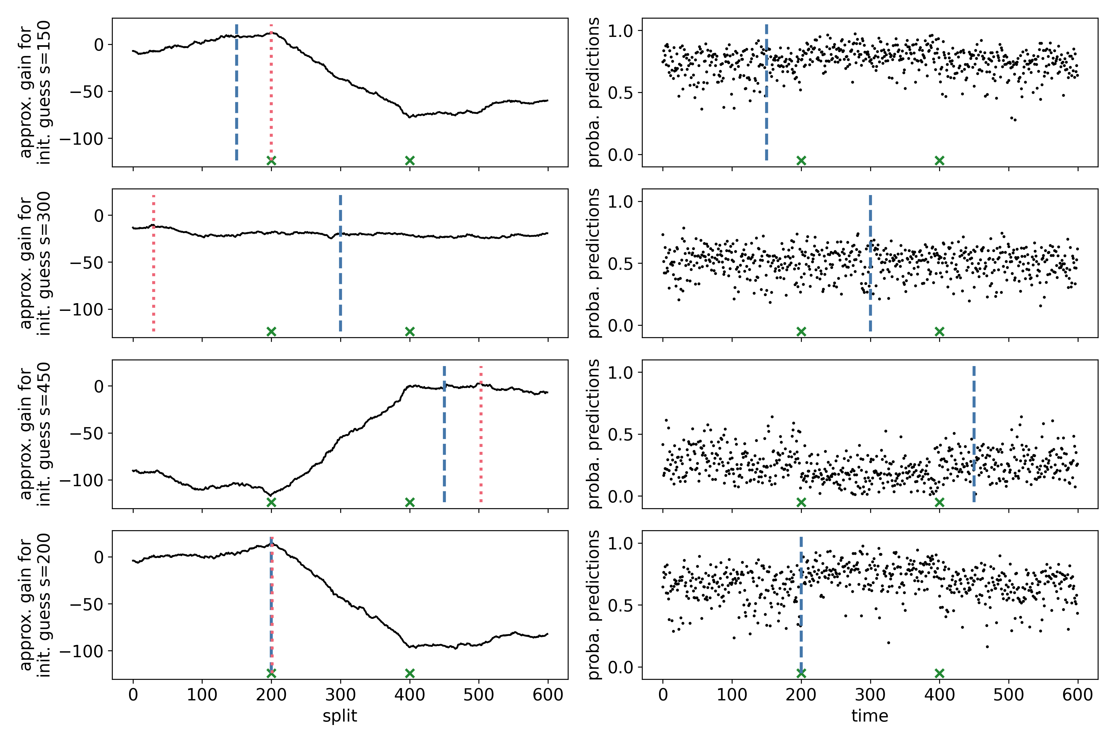
The figure below is based on a synthetic dataset with change points at $t = 200, 400$. The distributions of the first and last segment are equal. We assign a label 0 to observations left to the “first guess” (blue dashed line) and a label 1 to the right. The right panels contain the out-of-bag probability predictions of a random forest. These probability predictions yield classifier log-likelihood ratios, which aggregate to a “gain” in the left panel, similar to the CUSUM above. The first 3 panels contain gain curves for different “first guesses”. The last panel contains a gain curve using the maximizer of the first 3 gain curves as an initial guess.
The method is implemented in the changeforest software package available in R (conda-forge), Python (conda-forge and pypi), and Rust (crates.io).
Below is a video of a bee doing the “waggle dance” to communicate the direction and distance to a collection of pollen.
We fit changeforest on the differences of the green box’s x, y-coordinates, and angle for each frame.
In : changeforest(dX)
Out:                         best_split max_gain p_value
     (0, 180]                        41    9.793   0.005
      ¦--(0, 41]                     19   -3.148    0.36
      °--(41, 180]                  106    9.385   0.005
          ¦--(41, 106]               82   -3.831    0.16
          °--(106, 180]             153   21.758   0.005
              ¦--(106, 153]         124    0.314    0.08
              °--(153, 180]
The changeforest algorithm detects changepoints at $t=41, 106, 153$, corresponding to the time points where the bee changes between “waggling” and rotating.
Change point detection for graphical models in the presence of missing values
Londschien M., Kovács S. and Bühlmann P. (2021) Journal of Computational and Graphical Statistics
Most research in change point detection assumes the availability of complete observations. However, in many applications, some of the observations might be missing, with a missingness pattern that is not completely at random. This leads to a kind of “chicken and egg problem”: Missing values need to be imputed before standard change point methods can be applied. But, most imputation methods assume i.i.d. data, so to apply them, knowledge of the change points is required. When one imputes data as if the data was i.i.d., and if the missingness pattern is not missing completely at random, a subsequently applied change point algorithm possibly detects changes in the missingness pattern, not the underlying data.
We propose an approach that integrates the missingness directly into the change point detection loss function, assuming data is generated from a sparse Gaussian graphical model. We fit a covariance structure using the graphical Lasso. If, for a given segment, one variable has too many missing entries, we do not consider that variable.
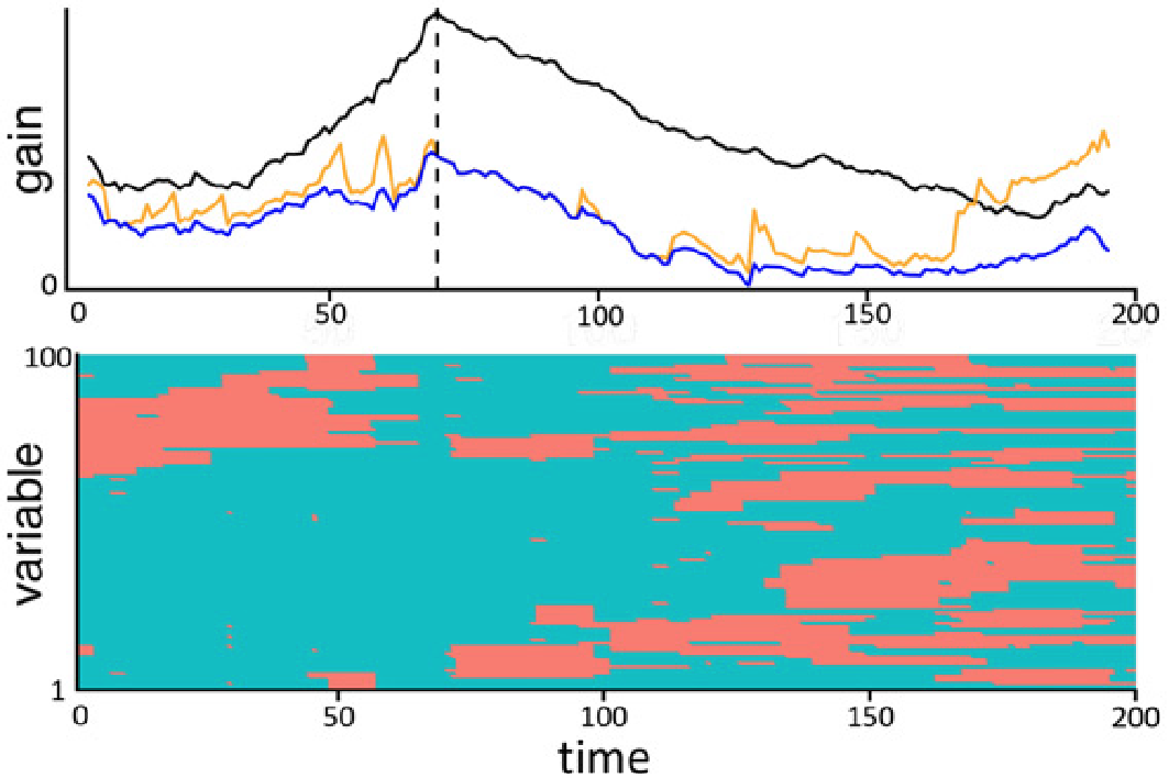
For the following data we simulated data with “blockwise missing” data, visualized in red on the bottom. The black line is the gain if the full data without missing values is used. The gain of the naive approach with simple imputation over the entire data is in orange. Our approach is in blue, with a maximum close to the true underlying change point (blue dashed vertical line).