In the lecture, you have seen various analyses for linear regression, e.g. standard errors of parameter estimates and p-values. Last exercise we saw that these analyses have different assumptions. For example, the OLS estimate is unbiased even for heteroscedastic errors. However, the derived standard deviations require homoscedasticity of the error terms. For the p-values to be exact, we furthermore require that the errors are normally distributed. However, we have seen that for a large sample size due to the CLT, the p-values are approximately correct even for non-normally distributed errors.
It is thus important to be able to verify model assumptions from data. This is typically done by visual inspection of model diagnostics plots. Two types of plots are popular in particular: The Tukey-Anscombe plot and the QQ plot.
A QQ (normal) plot plots the empirical quantiles of a sample against the theoretical quantiles of a normal distribution. The “QQ” stands for “quantile-quantile”. QQ plots are a tool to visually check whether data was drawn from a normal distribution. It can furthermore be used to analyze how the sampling distribution differs from a normal distribution. See this Stackexchange answer for an explanation of how to interpret QQ plots. Most importantly, the QQ plot can be used to measure the “heavy-tailedness” and the “skewness” of a distribution. See also this Shiny App from the same Stackexchange question.
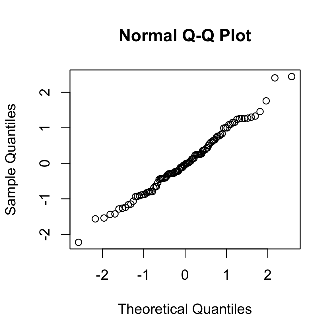
The following is a QQ (normal) plot of 100 i.i.d. samples from a standard Gaussian. The points lie approximately on the diagonal.
set.seed(0)
qqnorm(rnorm(100))
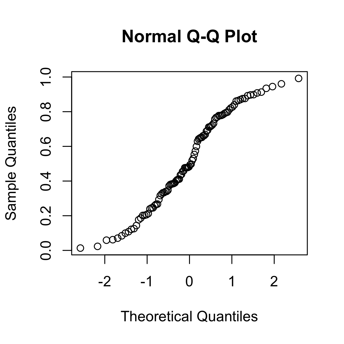
The following is a QQ (normal) plot of 100 i.i.d. samples from a uniform distribution. The uniform distribution has “shorter tails” than the Gaussian distribution (it is bounded).
set.seed(0)
qqnorm(runif(100))
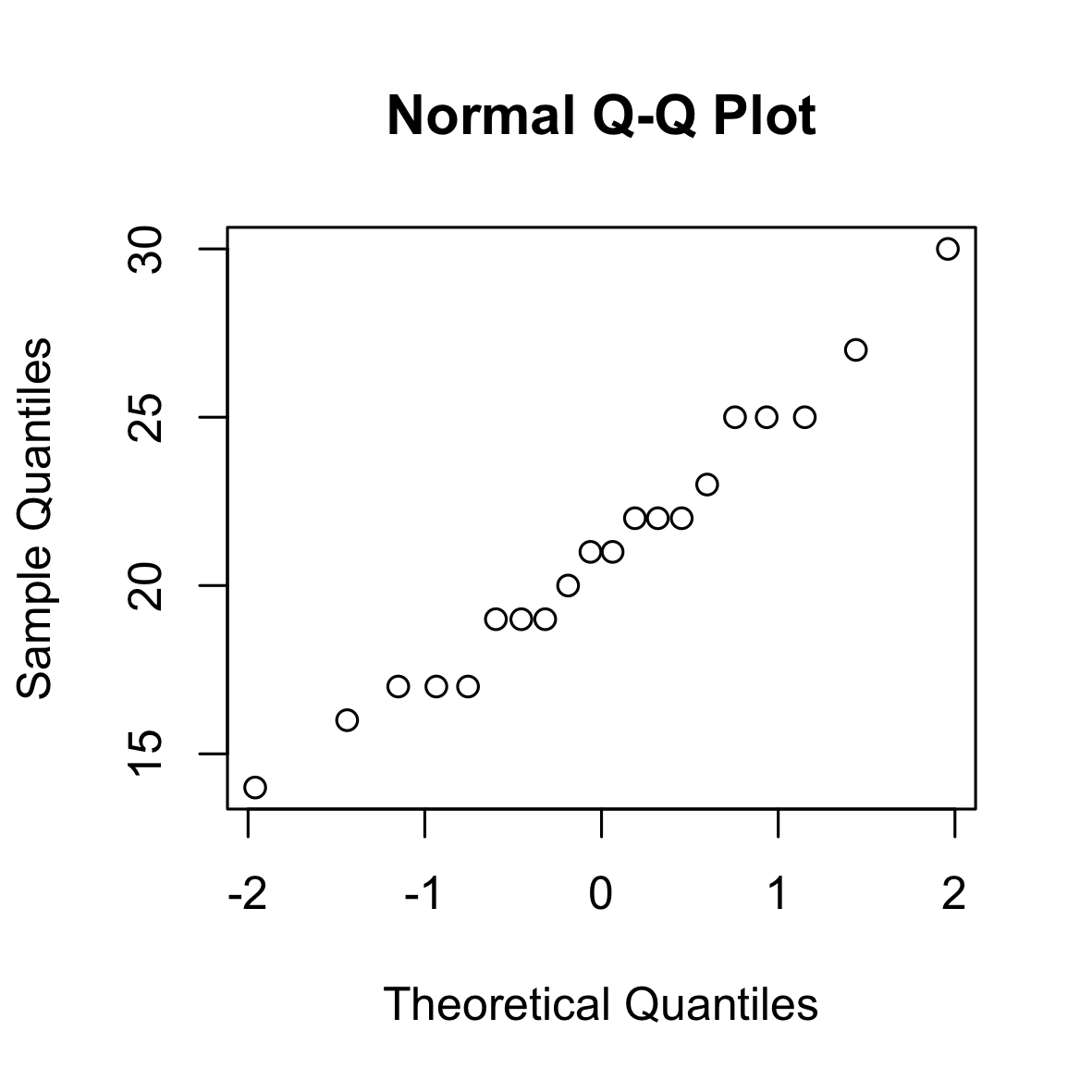
The following is a QQ (normal) plot of 100 i.i.d. samples from a binomial distribution. As the normal distribution approximates the binomial distribution, the points lie approximately on the diagonal.
set.seed(0)
qqnorm(rbinom(20, 100, 0.2))
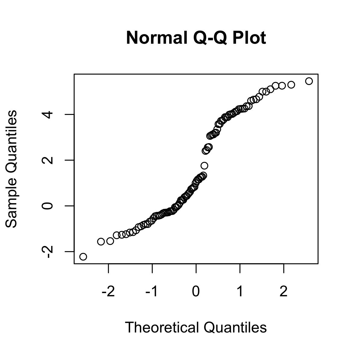
The following is a QQ (normal) plot of 100 i.i.d. samples from the mixture of two Gaussians. The bimodality of the Gaussian mixture leads to a “gap”.
set.seed(0)
qqnorm(c(rnorm(60), 4 + rnorm(40)))
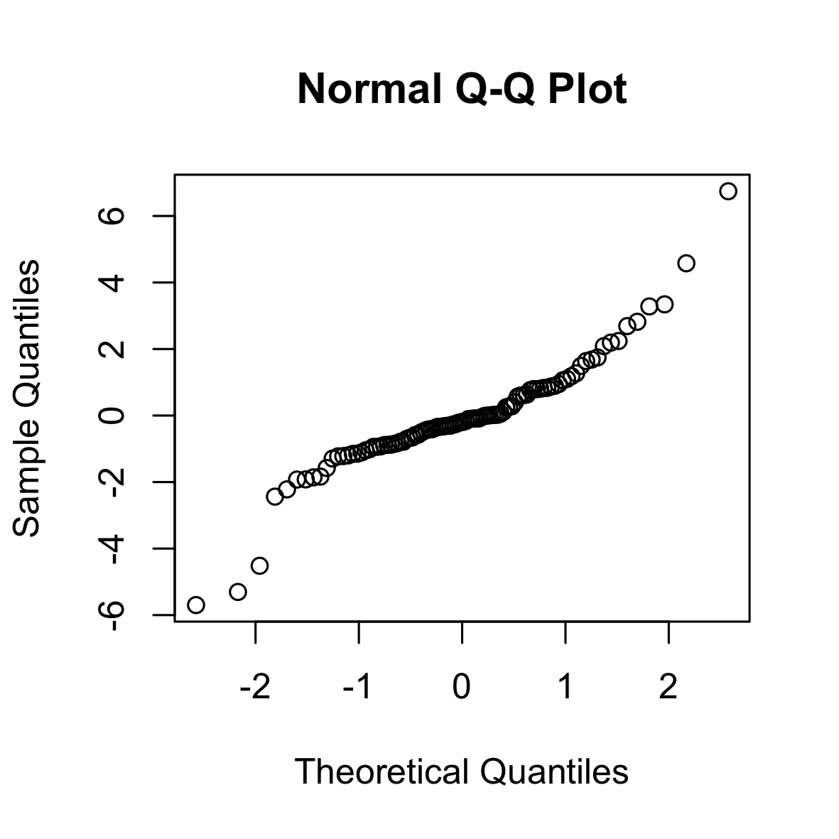
The following is a QQ (normal) plot of 100 i.i.d. samples from a Students-t-distribution with 4 degrees of freedom. The t-distribution has longer tails than the normal distribution.
set.seed(0)
qqnorm(rt(100, 4))
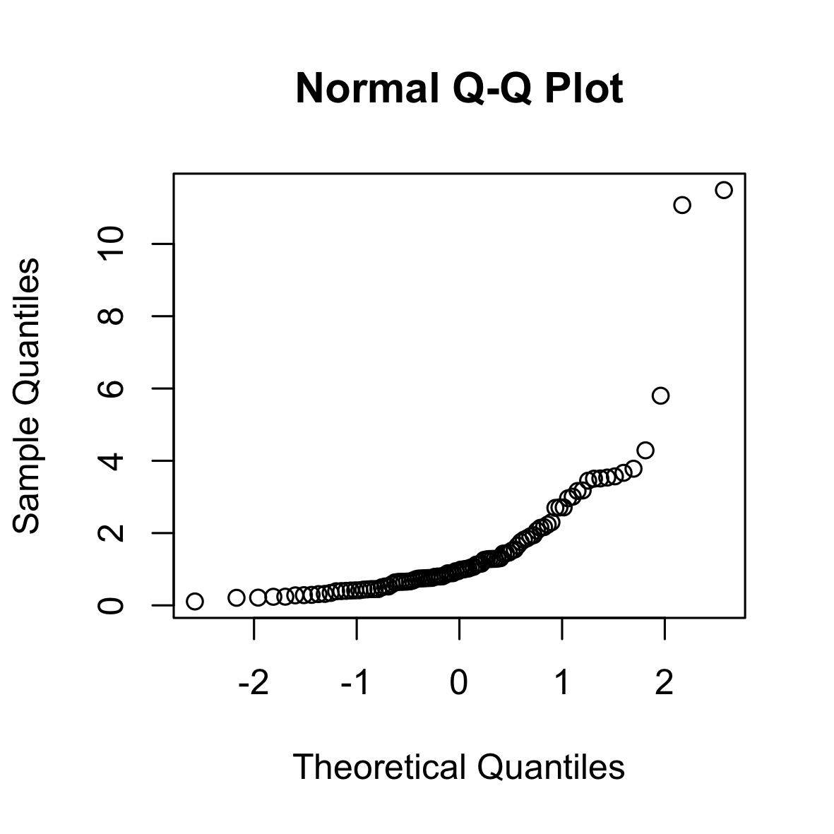
The following is a QQ (normal) plot of 100 i.i.d. samples from a log-normal distribution. The log-normal distribution is right-skewed and has longer tails than the normal distribution.
set.seed(0)
qqnorm(rlnorm(100))
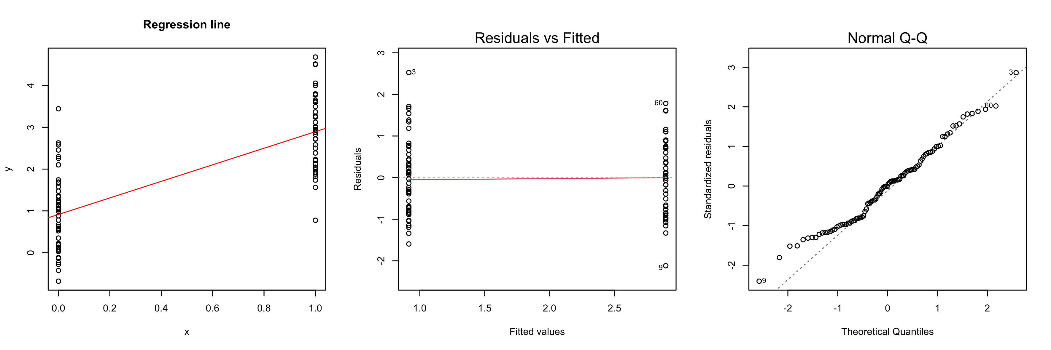
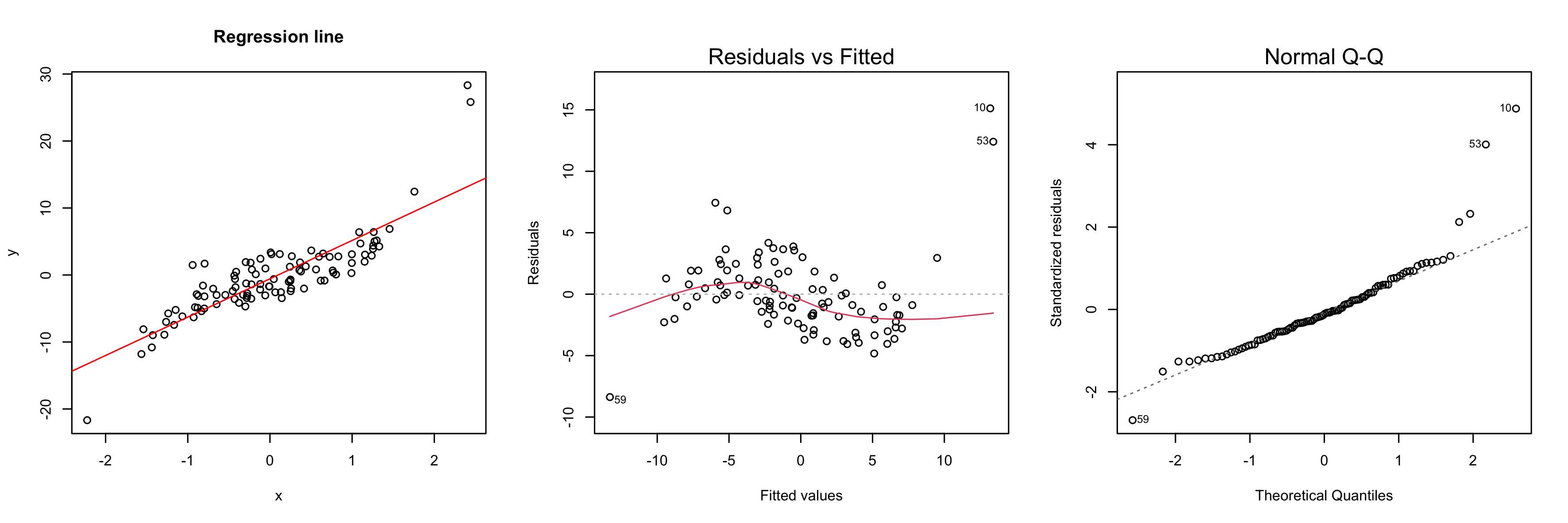
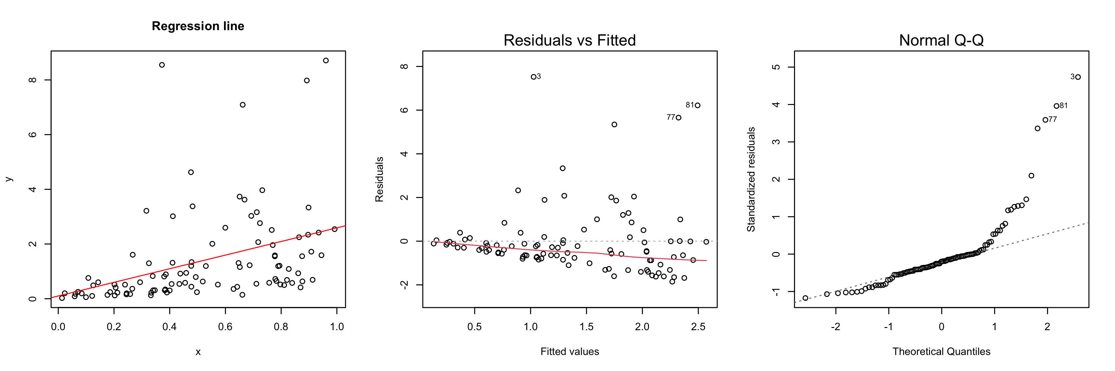
Another tool to verify model assumptions is the Tukey-Anscombe plot. In the Tukey-Anscombe plot, we plot residuals (y-axis) against fitted values. Optimally, the values fluctuate uniformly around the horizontal line at $y=0$. We can detect two model violations using the Tukey-Anscombe plot. (i) If the variance of the residuals appears to change with the fitted values, this is a sign of heteroscedasticity of the errors. A typical example where this is the case is when the errors are multiplicative, not additive. In such a case, a log-transformation stabilizes the variance of the errors. (ii) If the true regression function is not linear or we are missing a higher-order term, this will be reflected in the residuals. See the second plot below.
set.seed(0)
x <- rnorm(100)
y <- 2 * x + 0.5 * rnorm(100)

model <- lm(y ~ x)

par(mfrow=c(1,3))
plot(x, y)
title("Regression line")
lines(x, predict(model), col="red")
plot(model, which=1)
plot(model, which=2)

set.seed(0)
x <- rnorm(100)
y <- 2 * x + 1.5 * x ^ 3 - 0.7 + 2 * rnorm(100)

model <- lm(y ~ x)

par(mfrow=c(1,3))
plot(x, y)
title("Regression line")
abline(model, col="red")
plot(model, which=1)
plot(model, which=2)
set.seed(0)
x <- rnorm(100)
y <- 2 * x * rlnorm(100)

model <- lm(y ~ x)

par(mfrow=c(1,3))
plot(x, y)
title("Regression line")
abline(model, col="red")
plot(model, which=1)
plot(model, which=2)
set.seed(0)
x <- rbinom(1, 100)
y <- 2 * x + 1 + rnorm(100)

model <- lm(y ~ x)

par(mfrow=c(1,3))
plot(x, y)
title("Regression line")
abline(model, col="red")
plot(model, which=1)
plot(model, which=2)